

In this post, I explore the intricacies of Scaled Dot-Product Attention, a crucial attention mechanism integral to natural language processing (NLP) and deep learning. As Large Language Models (LLMs) like ChatGPT become increasingly prevalent, understanding the mechanisms behind attention has never been more important. These models leverage attention to discern and prioritize relevant information in vast sequences, enhancing both accuracy and efficiency. We'll delve deep into the Self-attention mechanism, particularly focusing on the Scaled Dot-Product Attention method, and elucidate its workings with visual aids to ensure a comprehensive grasp of this pivotal technology.
For those who favor a more dynamic and illustrative learning format, I've also produced an extensive video guide on Scaled Dot-Product Attention, now available on YouTube. Dive into the video for a detailed visual walk-through of how this attention mechanism transforms the landscape of NLP and deep learning.
Outline
Here's the structured breakdown of this article:
Introduction to Attention Mechanisms in NLP
Delving into Scaled Dot-Product Attention
Step-by-Step Walk-through of Scaled Dot-Product Attention
Concluding Thoughts
1. Introduction to Attention Mechanisms in NLP
Let's begin with an engaging example to understand the significance of the attention mechanism in NLP. Imagine the sentence:
"Under the starry sky, they set up camp and began to prepare for an evening of ___."
What might you predict to fill in the blank? Likely answers could include "storytelling," "rest," "music," or perhaps "dinner."
It's clear that unrelated words like "swimming," "conference," or "homework" wouldn't fit the context. This example underscores how attention helps models focus on relevant information to make contextually appropriate predictions.

Understanding the correct word hinges on the contextual clues and information woven through the preceding text. Language Models (LMs) are adept at predicting subsequent words by analyzing the surrounding context. Yet, for precise predictions, these models must grasp the intricate relationships between words in a sentence.
Enter the attention mechanism, a technique designed to spotlight the most pertinent words in a given context, thereby enhancing the model's predictive accuracy. In this discussion, we'll dive deep into the Scaled Dot-Product Attention mechanism, a potent method employed in deep learning for a variety of NLP tasks.
We'll break down its functionality, offer a detailed walkthrough with illustrative visuals, and present a simplified rendition of self-attention using PyTorch. To visually depict word relationships, consider a sentence where each word is linked to another, creating a network of connections that highlight their interdependence, much like a graph with arrows illustrating the links between each word pair.
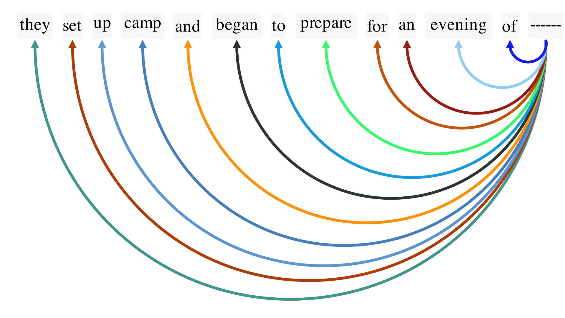
In the sentence, each word engages with others to varying extents, determined by the context and relational similarity. For instance, "starry" and "sky" or "camp" and "prepare" might share a stronger connection in our example, guiding the model to predict words related to outdoor activities or night-time settings. Next, we delve into the Scaled Dot-Product Attention mechanism in greater depth, elucidating how it leverages an attention matrix to discern and prioritize these word-to-word relationships effectively for accurate predictions.
2. Delving into Scaled Dot-Product Attention
Having established the attention mechanism's role in constructing a context similarity matrix, we now turn our focus to the Scaled Dot-Product Attention model. This model, a pivotal feature in the seminal work "Attention Is All You Need" by Vaswani et al., builds upon the existing concept of Dot-Product Attention. The introduction of a scaling factor, as delineated in this paper, markedly enhances the performance and effectiveness of the attention mechanism, setting a new standard for understanding and processing sequential data in neural networks.

It's important to note that the paper "Attention Is All You Need" by Vaswani et al. is renowned for introducing the Transformer architecture, marking a paradigm shift by applying the attention mechanism to feed-forward networks, whereas it was traditionally utilized in recurrent networks. While the broader implications of the Transformer are vast and influential, our focus here remains squarely on the Scaled Dot-Product Attention mechanism. A more thorough exploration of the Transformer architecture is reserved for a subsequent post.
The Scaled Dot-Product Attention mechanism operates by interacting with three matrices: a Query matrix (Q), a Key matrix (K), and a Value matrix (V). As depicted in the accompanying diagram, the process initiates by calculating the dot-product similarity between Q and K. This similarity matrix is then scaled down, and the Softmax function is applied to normalize these values, resulting in what is known as the attention matrix. The final step involves multiplying this attention matrix with the Value matrix (V), culminating in the output that reflects the weighted importance of each word or feature.
In the following section, we'll break down these steps comprehensively, detailing how the Query, Key, and Value matrices come into play and contribute to the mechanism's overall functionality.
Generating Query, Key, and Value Matrices
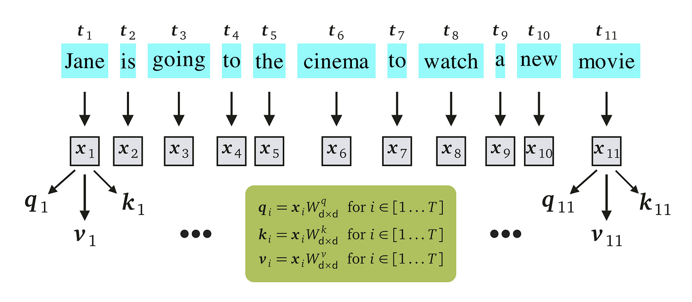
To understand how the query, key, and value vectors are derived, let's consider the input sequence has undergone preliminary processing through layers like an embedding layer, resulting in feature vectors x₁ through x₁₁. These feature vectors represent the sequence, each with a dimensionality of 1 by d, forming a matrix X of size 11 by d when concatenated.
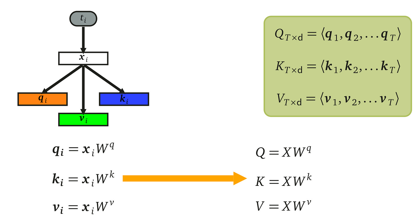
Each feature vector xᵢ from this matrix is then transformed through separate matrix multiplications with three distinct but learnable weight matrices. This transformation produces the respective qᵢ, kᵢ, and vᵢ vectors for each feature. Typically, the dimensions of the query (q) and key (k) vectors are identical and denoted as dₖ, allowing for compatibility in subsequent dot-product calculations. On the other hand, the dimension of the value (v) vector, denoted as dᵥ, can vary but is often set equal to the others for simplicity and uniformity, leading to a common dimensionality d = dₖ = dᵥ for all vectors. This standardization simplifies the architecture and tracking of dimensions throughout the model.

This simplificaiton ensures that the dot product computed between the query and key vectors yields a matrix of appropriate dimensions. . These weights are then applied to the value vectors to produce a weighted sum, effectively capturing the relevant information and reflecting the importance of each part of the input sequence in the context of the given task. This process is central to determining the focus of the attention mechanism on specific elements within the sequence.
The three weight matrices, responsible for transforming the input features into query, key, and value vectors, are learnable parameters of dimensions d×d. These matrices are applied consistently across the entire input sequence X, ensuring uniform transformation for each element. While it's possible to compute qᵢ, kᵢ, and vᵢ for each feature xᵢ individually from i=1 to i=11, a more efficient approach is to apply these weight matrices to the entire sequence X in one go. This method allows for batch processing of the sequence, leveraging matrix multiplication for faster and more efficient computation while maintaining the integrity of the transformation process.
A Simplified Implementation
In the upcoming code block, we embark on a journey to implement self-attention using PyTorch, starting with a straightforward example. For this initial setup, let's assume that our token IDs are ready — perhaps derived from tokenizing a sentence. Thus, we begin with these given token_ids:
import torch

token_ids  = [0,  5,  4,   9,  7,    2,   9,  10, 1,  6,   3]
token_ids = torch.tensor(token_ids, dtype=torch.int64)
Next, we will construct an Embedding layer to transform the token_ids into corresponding feature vectors:
torch.manual_seed(42)

vocab_size = 2000  # assume the number of unique vocabularies
d_model = 32       # dimensionality of feature vectors

embedding = torch.nn.Embedding(vocab_size, d_model)
X = embedding(token_ids)
print(X.shape)

## output:
torch.Size([11, 32])
With our initial setup complete, we now proceed to the attention layer. Here, we'll compute the Query (Q), Key (K), and Value (V) matrices:
torch.manual_seed(42)

W_q = torch.randn(d_model, d_model)
W_k = torch.randn(d_model, d_model)
W_v = torch.randn(d_model, d_model)

Q = X.matmul(W_q)
K = X.matmul(W_k)
V = X.matmul(W_v)

print(f'Q: {Q.shape}')
print(f'K: {K.shape}')
print(f'V: {V.shape}')

## output:
Q: torch.Size([11, 32])
K: torch.Size([11, 32])
V: torch.Size([11, 32])
In the following section, we'll delve into the process of deriving the query, key, and value vectors and explore their integral roles within the Scaled Dot-Product Attention mechanism.
3. Step-by-Step Walk-through of Scaled Dot-Product Attention
Step 1: Dot-Product Between Query and Key Matrices
The initial step in the Scaled Dot-Product Attention process is to compute the dot product between vector qᵢ (the query) and vector kⱼ (the key). To perform a dot product, it's necessary for the first vector to be a row vector and the second a column vector. This necessitates the transposition of vector kⱼ to form a column vector of dimensionality d×1. Executing this dot product yields a scalar value, representing the degree of similarity or 'attention' between the elements, as illustrated on the right.

This procedure is iteratively applied for all values of i and j, ranging from 1 to T. Upon completion, we acquire a comprehensive similarity matrix, also referred to as a compatibility matrix by the authors. As a more efficient alternative, this entire process can be expedited by employing matrix multiplication to calculate the entire compatibility matrix in one go. This method streamlines the computation, allowing for the simultaneous processing of all the pairwise dot products between the query and key vectors.
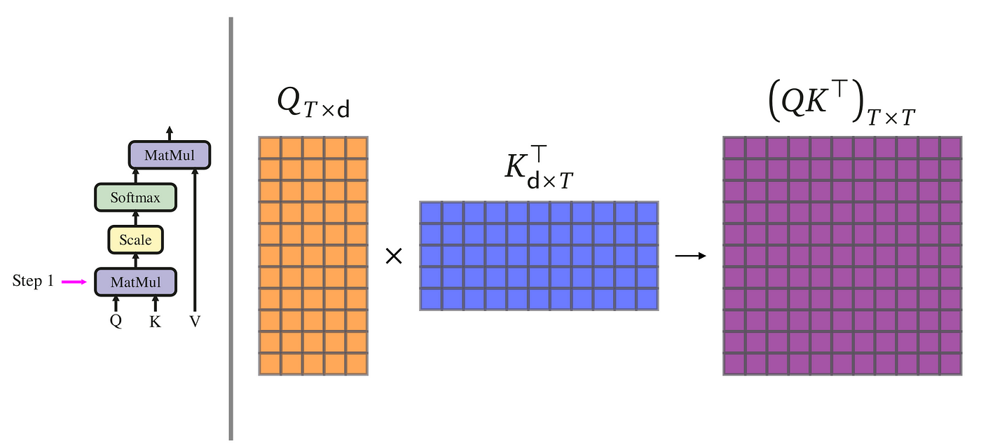
The similarity matrix effectively encapsulates the degree of similarity between each query and key vector pair, serving as an indicator for the amount of attention that should be allocated to each corresponding value vector in the input sequence. This crucial step can be efficiently implemented utilizing the matmul() function in PyTorch, which performs matrix multiplication as illustrated in the following example:
compat = Q.matmul(K.T)
print(compat.shape)

## Output:
torch.Size([11, 11])
In the provided code, K.T transposes matrix K to ensure the proper dimensions align for the dot-product computation. Moving forward, the next section will detail how this similarity matrix is refined through scaling and normalization using the Softmax function, which yields the final attention weights.
Step 2: Scaling the Compatibility Matrix
The subsequent step involves scaling the dot-products between the query and key vectors. This is achieved by dividing each element by the factor 1/√dₖ, where dₖ is the dimensionality of the key vectors. This scaling is critical for adjusting the range of the dot-products, ensuring stable gradients and a more controlled distribution of the attention scores.

It's pivotal to recognize that within the literature, attention mechanisms are broadly categorized into two types: multiplicative attention, including this dot-product attention, and additive attention. While additive attention isn't the focus of this discussion, it's noteworthy to mention that dot-product attention is typically more efficient computationally, and both types yield similar performance when the dimension d is modest. However, for larger dimensions of d, dot-product attention, if not scaled, tends to underperform compared to additive attention.
The authors of "Attention Is All You Need" suggest that the diminished performance of unscaled dot-product attention is due to an increase in variance. Specifically, if both queries and keys are initially normally distributed with zero mean and unit variance, the variance of their dot product escalates to d, corresponding to the dimensionality of the vectors. As d becomes large, so does the variance, propelling the output of the Softmax function into regions where gradients are minimal—akin to the vanishing gradients phenomenon in neural networks.
To illustrate the importance of scaling in mitigating this issue, the upcoming code block will apply scaling to the previously computed compatibility matrix. We will then visualize the effects by comparing heatmaps of the compatibility matrix before and after applying the scaling factor. This visual aid underscores the significant impact scaling has on the distribution and stability of attention scores.
import math

# scaling the matrix
scaled_compat = 1.0/math.sqrt(d_model) * compat

# plotting the heatmaps:
import matplotlib.pyplot as plt
import seaborn as sns

fig = plt.figure(figsize=(14, 10))
ax = fig.add_axes((0.05, 0.05, 0.45, 0.45))
sns.heatmap(compat.detach().numpy(), cmap='coolwarm')
ax.set_title(r'$QK^\top$', size=15)
ax = fig.add_axes((0.55, 0.05, 0.45, 0.45))
sns.heatmap(scaled_compat.detach().numpy(), cmap='coolwarm')
ax.set_title(r'After scaling: $\frac{1}{\sqrt{d}}QK^\top$', size=15)
plt.show()
print(f'Variance of Q: {torch.var(Q).item():.2f}')
print(f'Variance of K: {torch.var(K).item():.2f}')
print(f'Variance of compatib. matrix (before scaling): {torch.var(compat).item():.2f}')
print(f'Variance of compatib. matrix (after scaling): {torch.var(scaled_compat).item():.2f}')

## output:
Variance of Q: 34.12
Variance of K: 26.70
Variance of compatib. matrix (before scaling): 25801.72
Variance of compatib. matrix (after scaling): 806.30
As illustrated, the variance of Q and K vectors are approximately 34 and 26, respectively. However, after the dot-product operation, the variance surges to approximately 25801. Scaling is thus essential to mitigate this dramatic increase in variance, which is crucial for stabilizing the subsequent application of the Softmax function.
Step 3: Obtaining Attention Weights with Softmax Normalization
In the third step, we proceed by applying the Softmax function to the scaled compatibility matrix. As a quick refresher, the Softmax function is a normalization technique that converts a vector z of arbitrary real values into a probability distribution of n values. Each component σ(zᵢ) of the output vector [σ(z₁), ..., σ(zₙ)] is computed using the equation:
This transformation ensures that each element of the resulting vector is between 0 and 1, with the entire vector summing to 1. This property is incredibly useful in converting the scaled compatibility scores into a set of attention weights that effectively represent probabilities or the relative importance of each value in the input sequence. In the subsequent section, we will see how these attention weights are then used to produce a weighted sum of value vectors, ultimately forming the output of the attention mechanism.
The Softmax function is characterized by two critical properties:
Each output falls between zero and one: This ensures that every element of the transformed vector is a valid probability, reflecting the relative importance or attention assigned to each input element.
\(0\le \sigma(z_i) \le 1 \text{ for } i=0\text{ to }n\)The sum of all the outputs is 1: This property guarantees that the transformed outputs form a probability distribution, meaning the entire set of weights for any given input sums to unity.
\(\sum_{j=1}^n \sigma(z_j) = 1\)
Therefore, in step 3, we apply the Softmax function to each row of the scaled compatibility matrix. This operation yields a matrix of attention weights, where the sum of weights in each row is exactly 1. This matrix effectively represents the distribution of attention across the inputs, with each row corresponding to the attention distribution for a particular query.

In PyTorch, this transformation can be efficiently achieved with the following code:
attention = torch.softmax(scaled_compat, dim=0)
print(attention.shape)
## output:
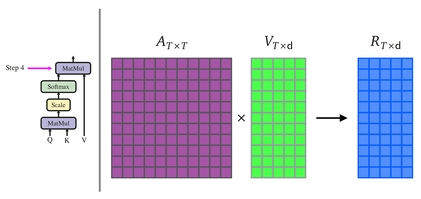
torch.Size([11, 11])Step 4: Generating the Context Vectors as the Final Output
In the final stage of the Scaled Dot-Product Attention mechanism, we utilize the previously calculated attention matrix, denoted as A with dimensions T×T, along with the value matrix V, dimensioned T×d. By conducting matrix multiplication of A×V, we derive a new matrix also of dimensions T×d.
In this step, there's no need for transposition, as the dimensions of A and V naturally align for multiplication. The product of this operation is what we refer to as the context matrix. It encapsulates the final output of our attention layer, comprising d-dimensional vectors. Each vector within this context matrix embodies the aggregated context for each corresponding token in the input sequence, effectively summarizing the relevant information as directed by the attention weights.
The following code block implements this final step, multiplying the attention matrix with the value matrix to yield the context vectors:
results = attention.matmul(V)

print(results.shape)

## output:
torch.Size([11, 32])
This outputs a matrix with dimensions 11x32, representing the context vectors for each token in our input sequence.
4. Concluding Thoughts
In this comprehensive guide, we've journeyed through the intricacies of the scaled dot-product attention mechanism, a fundamental building block in the architecture of contemporary deep learning models, particularly transformers. Our discussion began with an exploration of the pivotal role of attention mechanisms in natural language processing, highlighting their capability to discern and emphasize the intricate relationships between words in a sentence. We then embarked on a detailed walkthrough of the scaled dot-product attention process, breaking down each step: from computing the query, key, and value vectors, creating the compatibility matrix, normalizing with Softmax, to finally constructing the context vector.
In addition to theoretical insights, we provided a hands-on implementation using PyTorch, offering a practical perspective on this powerful attention mechanism. This deeper understanding equips readers with a clearer appreciation of the sophistication and adaptability of modern deep learning models, as well as the critical role attention mechanisms play in pushing the boundaries of natural language processing tasks.
As we conclude this article, we pave the way for an upcoming exploration into multi-head attention, an evolution of the mechanisms discussed here. Multi-head attention allows the model to capture information from different representation subspaces at different positions, offering a more nuanced and comprehensive understanding of context. This next piece will delve into the architecture and advantages of multi-head attention, demonstrating how it further enhances the capabilities and performance of models like Transformers. Stay tuned for an exciting continuation of our journey into the depths of attention mechanisms and their transformative impact on the field of AI and NLP.
Awesome write-up!